Gaussian Distribution Example
import tensorflow_probability as tfp

tfd = tfp.distributions
import matplotlib.pyplot as plt
import tensorflow as tf
import seaborn as sns
import numpy as np
import scipy
import tqdm
import maxent
import os

tf.random.set_seed(0)
np.random.seed(0)
os.environ["CUDA_VISIBLE_DEVICES"] = "-1"
sns.set_context("paper")
sns.set_style(
    "whitegrid",
    {
        "xtick.bottom": True,
        "ytick.left": True,
        "xtick.color": "#333333",
        "ytick.color": "#333333",
    },
)
# plt.rcParams["font.family"] = "serif"
plt.rcParams["mathtext.fontset"] = "dejavuserif"
colors = ["#1b9e77", "#d95f02", "#7570b3", "#e7298a", "#66a61e"]
%matplotlib inline
Set-up Prior Distribution
x = np.array([1.0, 1.0])
i = tf.keras.Input((1,))
l = maxent.TrainableInputLayer(x)(i)
d = tfp.layers.DistributionLambda(
    lambda x: tfd.Normal(loc=x[..., 0], scale=tf.math.exp(x[..., 1]))
)(l)
model = maxent.ParameterJoint([lambda x: x], inputs=i, outputs=[d])
model.compile(tf.keras.optimizers.Adam(0.1))
model(tf.constant([1.0]))
<tfp.distributions._TensorCoercible 'tensor_coercible' batch_shape=[1] event_shape=[] dtype=float32>
Simulator
def simulate(x):
    y = np.random.normal(loc=x, scale=0.1)
    return y


plt.figure()
unbiased_params = model.sample(100000)
y = simulate(*unbiased_params)
y = np.squeeze(y)
<Figure size 432x288 with 0 Axes>
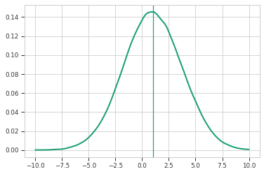
pdf = scipy.stats.gaussian_kde(y)
x = np.linspace(-10, 10, 100)
plt.plot(x, pdf.pdf(x), color=colors[0], linewidth=2)
plt.axvline(np.mean(y), color=colors[0])
<matplotlib.lines.Line2D at 0x7ff3b490a400>
Maximum Entropy Method
r = maxent.Restraint(lambda x: x, 4, maxent.EmptyPrior())
me_model = maxent.MaxentModel([r])
me_model.compile(tf.keras.optimizers.Adam(0.01), "mean_squared_error")
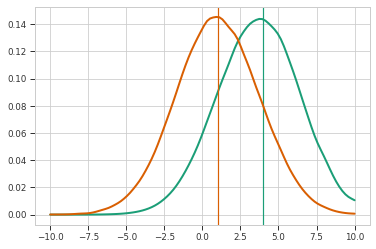
result = me_model.fit(y, epochs=4, batch_size=128)
plt.axvline(x=4, color=colors[0])
wpdf = scipy.stats.gaussian_kde(
    np.squeeze(y), weights=np.squeeze(me_model.traj_weights)
)
x = np.linspace(-10, 10, 100)
plt.plot(x, wpdf.pdf(x), color=colors[0], linewidth=2)


plt.plot(x, pdf.pdf(x), color=colors[1], linewidth=2)
plt.axvline(np.mean(np.squeeze(y)), color=colors[1])
<matplotlib.lines.Line2D at 0x7ff33c74ed00>
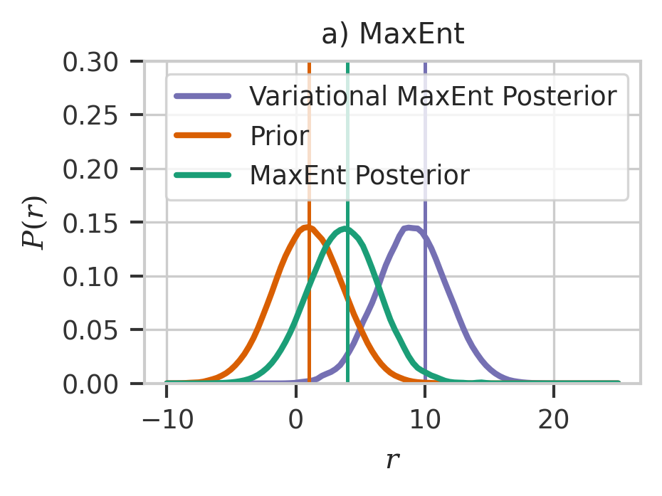
Variational MaxEnt
Try to fit to more extreme value - 10
r = maxent.Restraint(lambda x: x, 10, maxent.EmptyPrior())
hme_model = maxent.HyperMaxentModel([r], model, simulate)
hme_model.compile(tf.keras.optimizers.SGD(0.005), "mean_squared_error")
result = hme_model.fit(epochs=4, sample_batch_size=len(y) // 4, verbose=0)
WARNING:tensorflow:Gradients do not exist for variables ['value:0'] when minimizing the loss. If you're using `model.compile()`, did you forget to provide a `loss`argument?
WARNING:tensorflow:Gradients do not exist for variables ['value:0'] when minimizing the loss. If you're using `model.compile()`, did you forget to provide a `loss`argument?
WARNING:tensorflow:Gradients do not exist for variables ['value:0'] when minimizing the loss. If you're using `model.compile()`, did you forget to provide a `loss`argument?
w2pdf = scipy.stats.gaussian_kde(
    np.squeeze(hme_model.trajs), weights=np.squeeze(hme_model.traj_weights)
)
plt.figure(figsize=(3, 2), dpi=300)
x = np.linspace(-10, 25, 100)
plt.plot(
    x, w2pdf.pdf(x), color=colors[2], linewidth=2, label="Variational MaxEnt Posterior"
)
plt.axvline(x=10, color=colors[2])

plt.plot(x, pdf.pdf(x), color=colors[1], linewidth=2, label="Prior")
plt.axvline(np.mean(np.squeeze(y)), color=colors[1])

plt.plot(x, wpdf.pdf(x), color=colors[0], linewidth=2, label="MaxEnt Posterior")
plt.axvline(x=4, color=colors[0])
plt.ylim(0, 0.30)
plt.xlabel(r"$r$")
plt.ylabel(r"$P(r)$")
plt.title("a) MaxEnt")
plt.legend()
plt.savefig("maxent.svg")
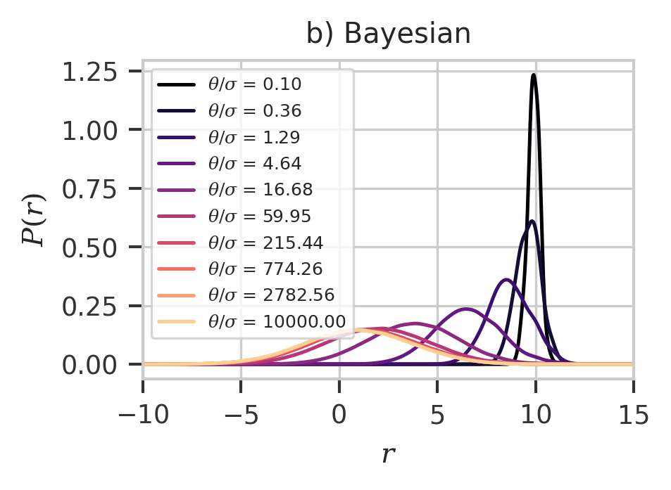
Bayesian Inference Setting
# https://pubmed.ncbi.nlm.nih.gov/26723635/
plt.figure(figsize=(3, 2), dpi=300)
x = np.linspace(-10, 25, 1000)
cmap = plt.get_cmap("magma")
prior_theta = 10 ** np.linspace(-1, 4, 10)
bpdf = np.exp(-((y - 10) ** 2) / (2 * prior_theta[:, np.newaxis]))
bpdf /= np.sum(bpdf, axis=1)[:, np.newaxis]
for i, p in enumerate(prior_theta):
    ppdf = scipy.stats.gaussian_kde(np.squeeze(y), weights=bpdf[i])
    plt.plot(
        x,
        ppdf.pdf(x),
        color=cmap(i / len(prior_theta)),
        label=f"$\\theta/\\sigma$ = {p:.2f}",
    )
plt.legend(fontsize=6)
plt.xlim(-10, 15)
plt.xlabel(r"$r$")
plt.ylabel(r"$P(r)$")
plt.title("b) Bayesian")
plt.savefig("bayes.svg")
plt.show()
Effects of Observable
bayesian_results = []
# scipy.stats.wasserstein_distance(y, y, u_weights=np.ones_like(y) / len(y), v_weights=bpdf[i])])
x2 = np.linspace(-20, 20, 10000)
for i in range(len(prior_theta)):
    ppdf = scipy.stats.gaussian_kde(np.squeeze(y), weights=bpdf[i])
    bayesian_results.append(
        [
            np.sum(ppdf.pdf(x) * x * (x[1] - x[0])),
            -np.nansum((x[1] - x[0]) * ppdf.pdf(x) * np.log(ppdf.pdf(x))),
        ]
    )
    print(i, bayesian_results[-1])
/tmp/ipykernel_2791/2902584349.py:9: RuntimeWarning: divide by zero encountered in log
  -np.nansum((x[1] - x[0]) * ppdf.pdf(x) * np.log(ppdf.pdf(x))),
/tmp/ipykernel_2791/2902584349.py:9: RuntimeWarning: invalid value encountered in multiply
  -np.nansum((x[1] - x[0]) * ppdf.pdf(x) * np.log(ppdf.pdf(x))),
0 [9.911016359048261, 0.3042573578163087]
1 [9.631094028403169, 0.9771244951498036]
2 [8.674678518807875, 1.5288348252198853]
3 [6.52612859002079, 1.9553957761896448]
4 [3.7846027053356988, 2.244649224089299]
5 [1.9951996500959486, 2.371265813381091]
6 [1.2995967637152959, 2.4118962049488717]
7 [1.0843316455584768, 2.423766089350074]
8 [1.022553823634384, 2.427114909604028]
9 [1.005213548622557, 2.428050282245948]
me_results = []
for i in range(-5, 10):
    r = maxent.Restraint(lambda x: x, i, maxent.EmptyPrior())
    m = maxent.MaxentModel([r])
    m.compile(tf.keras.optimizers.Adam(0.001), "mean_squared_error")
    m.fit(y, epochs=4, batch_size=256, verbose=0)
    # d = scipy.stats.wasserstein_distance(y, y, u_weights=m.traj_weights)
    ppdf = scipy.stats.gaussian_kde(y, weights=m.traj_weights)
    d = -np.nansum((x[1] - x[0]) * ppdf.pdf(x) * np.log(ppdf.pdf(x)))
    me_results.append([i, d])
    print(np.sum(y * m.traj_weights), d)
-4.760423 2.3069205940095037
-3.8109474 2.3694516349941894
-2.8259637 2.403835068355486
-1.9008719 2.4184477783793352
-0.9553167 2.424371353211651
0.027614227 2.4268825734892565
/tmp/ipykernel_2791/1084787031.py:9: RuntimeWarning: divide by zero encountered in log
  d = -np.nansum((x[1] - x[0]) * ppdf.pdf(x) * np.log(ppdf.pdf(x)))
/tmp/ipykernel_2791/1084787031.py:9: RuntimeWarning: invalid value encountered in multiply
  d = -np.nansum((x[1] - x[0]) * ppdf.pdf(x) * np.log(ppdf.pdf(x)))
1.0098245 2.428427371218406
1.9941295 2.4295492555818403
2.9686315 2.4306696969756376
3.8970127 2.433814611080603
4.834799 2.443655280630767
5.8534675 2.4694963819727938
6.846133 2.51482597869503
7.641946 2.5621808310126912
8.217658 2.5977537752590063
plt.figure(figsize=(3, 2), dpi=300)
me_result = np.array(me_results)
bayesian_results = np.array(bayesian_results)
plt.plot(me_result[:, 0], me_result[:, 1], label="MaxEnt", color=colors[0])
plt.plot(
bayesian_results[:, 0],
bayesian_results[:, 1],
linestyle="--",
label="Bayesian Inference",
color=colors[1],
)
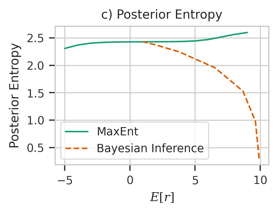
plt.ylabel("Posterior Entropy")
plt.xlabel("$E[r]$")
plt.legend()
plt.title("c) Posterior Entropy")
plt.savefig("post.svg")
plt.show()
bayesian_results[:]
array([[9.91101636, 0.30425736],
       [9.63109403, 0.9771245 ],
       [8.67467852, 1.52883483],
       [6.52612859, 1.95539578],
       [3.78460271, 2.24464922],
       [1.99519965, 2.37126581],
       [1.29959676, 2.4118962 ],
       [1.08433165, 2.42376609],
       [1.02255382, 2.42711491],
       [1.00521355, 2.42805028]])