LIME paper: Recurrent Neural Network for Solubility Prediciton

Import packages and set up RNN

import pandas as pd
import matplotlib.pyplot as plt
import matplotlib as mpl
import numpy as np
import tensorflow as tf
import selfies as sf
import exmol
from dataclasses import dataclass
from rdkit.Chem.Draw import rdDepictor, MolsToGridImage
from rdkit.Chem import MolFromSmiles
import random
rdDepictor.SetPreferCoordGen(True)
import matplotlib.pyplot as plt
import matplotlib.font_manager as font_manager
import urllib.request

urllib.request.urlretrieve(
    "https://github.com/google/fonts/raw/main/ofl/ibmplexmono/IBMPlexMono-Regular.ttf",
    "IBMPlexMono-Regular.ttf",
)
fe = font_manager.FontEntry(fname="IBMPlexMono-Regular.ttf", name="plexmono")
font_manager.fontManager.ttflist.append(fe)
plt.rcParams.update(
    {
        "axes.facecolor": "#f5f4e9",
        "grid.color": "#AAAAAA",
        "axes.edgecolor": "#333333",
        "figure.facecolor": "#FFFFFF",
        "axes.grid": False,
        "axes.prop_cycle": plt.cycler("color", plt.cm.Dark2.colors),
        "font.family": fe.name,
        "figure.figsize": (3.5, 3.5 / 1.2),
        "ytick.left": True,
        "xtick.bottom": True,
    }
)
mpl.rcParams["font.size"] = 12
soldata = pd.read_csv(
    "https://github.com/whitead/dmol-book/raw/main/data/curated-solubility-dataset.csv"
)

features_start_at = list(soldata.columns).index("MolWt")
np.random.seed(0)
random.seed(0)

2025-04-06 12:55:27.166914: I external/local_xla/xla/tsl/cuda/cudart_stub.cc:32] Could not find cuda drivers on your machine, GPU will not be used.
2025-04-06 12:55:27.170336: I external/local_xla/xla/tsl/cuda/cudart_stub.cc:32] Could not find cuda drivers on your machine, GPU will not be used.
2025-04-06 12:55:27.179096: E external/local_xla/xla/stream_executor/cuda/cuda_fft.cc:467] Unable to register cuFFT factory: Attempting to register factory for plugin cuFFT when one has already been registered
WARNING: All log messages before absl::InitializeLog() is called are written to STDERR
E0000 00:00:1743944127.193324   41935 cuda_dnn.cc:8579] Unable to register cuDNN factory: Attempting to register factory for plugin cuDNN when one has already been registered
E0000 00:00:1743944127.197737   41935 cuda_blas.cc:1407] Unable to register cuBLAS factory: Attempting to register factory for plugin cuBLAS when one has already been registered
W0000 00:00:1743944127.209683   41935 computation_placer.cc:177] computation placer already registered. Please check linkage and avoid linking the same target more than once.
W0000 00:00:1743944127.209694   41935 computation_placer.cc:177] computation placer already registered. Please check linkage and avoid linking the same target more than once.
W0000 00:00:1743944127.209696   41935 computation_placer.cc:177] computation placer already registered. Please check linkage and avoid linking the same target more than once.
W0000 00:00:1743944127.209698   41935 computation_placer.cc:177] computation placer already registered. Please check linkage and avoid linking the same target more than once.
2025-04-06 12:55:27.213998: I tensorflow/core/platform/cpu_feature_guard.cc:210] This TensorFlow binary is optimized to use available CPU instructions in performance-critical operations.
To enable the following instructions: AVX2 FMA, in other operations, rebuild TensorFlow with the appropriate compiler flags.

# scramble them
soldata = soldata.sample(frac=0.01, random_state=0).reset_index(drop=True)
soldata.head()

	ID	Name	InChI	InChIKey	SMILES	Solubility	SD	Ocurrences	Group	MolWt	...	NumRotatableBonds	NumValenceElectrons	NumAromaticRings	NumSaturatedRings	NumAliphaticRings	RingCount	TPSA	LabuteASA	BalabanJ	BertzCT
0	B-4206	diuron	InChI=1S/C9H10Cl2N2O/c1-13(2)9(14)12-6-3-4-7(1...	XMTQQYYKAHVGBJ-UHFFFAOYSA-N	CN(C)C(=O)Nc1ccc(Cl)c(Cl)c1	-3.744300	1.227164	5	G4	233.098	...	1.0	76.0	1.0	0.0	0.0	1.0	32.34	92.603980	2.781208	352.665233
1	F-988	7-(3-amino-3-methylazetidin-1-yl)-8-chloro-1-c...	InChI=1S/C17H17ClFN3O3/c1-17(20)6-21(7-17)14-1...	DUNZFXZSFJLIKR-UHFFFAOYSA-N	CC1(N)CN(C2=C(Cl)C3=C(C=C2F)C(=O)C(C(=O)O)=CN3...	-5.330000	0.000000	1	G1	365.792	...	3.0	132.0	2.0	2.0	2.0	4.0	88.56	147.136366	2.001398	973.487509
2	C-1996	4-acetoxybiphenyl; 4-biphenylyl acetate	InChI=1S/C14H12O2/c1-11(15)16-14-9-7-13(8-10-1...	MISFQCBPASYYGV-UHFFFAOYSA-N	CC(=O)OC1=CC=C(C=C1)C2=CC=CC=C2	-4.400000	0.000000	1	G1	212.248	...	2.0	80.0	2.0	0.0	0.0	2.0	26.30	94.493449	2.228677	471.848345
3	A-3055	methane dimolybdenum	InChI=1S/CH4.2Mo/h1H4;;	JAGQSESDQXCFCH-UHFFFAOYSA-N	C.[Mo].[Mo]	-3.420275	0.409223	2	G3	207.923	...	0.0	20.0	0.0	0.0	0.0	0.0	0.00	49.515427	-0.000000	2.754888
4	A-2575	ethyl 4-[[(methylphenylamino)methylene]amino]b...	InChI=1S/C17H18N2O2/c1-3-21-17(20)14-9-11-15(1...	GNGYPJUKIKDJQT-UHFFFAOYSA-N	CCOC(=O)c1ccc(cc1)N=CN(C)c2ccccc2	-5.450777	0.000000	1	G1	282.343	...	5.0	108.0	2.0	0.0	0.0	2.0	41.90	124.243431	2.028889	606.447052

5 rows × 26 columns

from rdkit.Chem import MolToSmiles


def _randomize_smiles(mol, isomericSmiles=True):
    return MolToSmiles(
        mol,
        canonical=False,
        doRandom=True,
        isomericSmiles=isomericSmiles,
        kekuleSmiles=random.random() < 0.5,
    )

smiles = list(soldata["SMILES"])
solubilities = list(soldata["Solubility"])

aug_data = 10


def largest_mol(smiles):
    ss = smiles.split(".")
    ss.sort(key=lambda a: len(a))
    return ss[-1]


aug_smiles = []
aug_solubilities = []
for sml, sol in zip(smiles, solubilities):
    sml = largest_mol(sml)
    if len(sml) <= 4:
        continue  # ion or metal
    new_smls = []
    new_smls.append(sml)
    aug_solubilities.append(sol)
    for _ in range(aug_data):
        try:
            new_sml = _randomize_smiles(MolFromSmiles(sml))
            if new_sml not in new_smls:
                new_smls.append(new_sml)
                aug_solubilities.append(sol)
        except:
            continue
    aug_smiles.extend(new_smls)

aug_df_AqSolDB = pd.DataFrame(
    data={"SMILES": aug_smiles, "Solubility": aug_solubilities}
)

print(f"The dataset was augmented from {len(soldata)} to {len(aug_df_AqSolDB)}.")

The dataset was augmented from 100 to 990.

selfies_list = []
for s in aug_df_AqSolDB.SMILES:
    try:
        selfies_list.append(sf.encoder(exmol.sanitize_smiles(s)[1]))
    except sf.EncoderError:
        selfies_list.append(None)
len(selfies_list)

990

basic = set(exmol.get_basic_alphabet())
data_vocab = set(
    sf.get_alphabet_from_selfies([s for s in selfies_list if s is not None])
)
vocab = ["[nop]"]
vocab.extend(list(data_vocab.union(basic)))
vocab_stoi = {o: i for o, i in zip(vocab, range(len(vocab)))}


def selfies2ints(s):
    result = []
    for token in sf.split_selfies(s):
        if token in vocab_stoi:
            result.append(vocab_stoi[token])
        else:
            result.append(np.nan)
            # print('Warning')
    return result


def ints2selfies(v):
    return "".join([vocab[i] for i in v])


# test them out
s = selfies_list[0]
print("selfies:", s)
v = selfies2ints(s)
print("selfies2ints:", v)
so = ints2selfies(v)

selfies: [C][N][Branch1][C][C][C][=Branch1][C][=O][N][C][=C][C][=C][Branch1][C][Cl][C][Branch1][C][Cl][=C][Ring1][Branch2]
selfies2ints: [9, 12, 38, 9, 9, 9, 32, 9, 46, 12, 9, 34, 9, 34, 38, 9, 5, 9, 38, 9, 5, 34, 33, 20]

# creating an object
@dataclass
class Config:
    vocab_size: int
    example_number: int
    batch_size: int
    buffer_size: int
    embedding_dim: int
    rnn_units: int
    hidden_dim: int
    drop_rate: float


config = Config(
    vocab_size=len(vocab),
    example_number=len(selfies_list),
    batch_size=128,
    buffer_size=10000,
    embedding_dim=64,
    hidden_dim=32,
    rnn_units=64,
    drop_rate=0.20,
)

# now get sequences
encoded = [selfies2ints(s) for s in selfies_list if s is not None]
# check for non-Nones
dsolubilities = aug_df_AqSolDB.Solubility.values[[s is not None for s in selfies_list]]
padded_seqs = tf.keras.preprocessing.sequence.pad_sequences(encoded, padding="post")

# Should be shuffled from the beginning, so no worries
N = len(padded_seqs)
split = int(0.1 * N)

# Now build dataset
test_data = tf.data.Dataset.from_tensor_slices(
    (padded_seqs[:split], dsolubilities[:split])
).batch(config.batch_size)

nontest = tf.data.Dataset.from_tensor_slices(
    (
        padded_seqs[split:],
        dsolubilities[split:],
    )
)
val_data, train_data = nontest.take(split).batch(config.batch_size), nontest.skip(
    split
).shuffle(config.buffer_size).batch(config.batch_size).prefetch(
    tf.data.experimental.AUTOTUNE
)

2025-04-06 12:55:31.574234: E external/local_xla/xla/stream_executor/cuda/cuda_platform.cc:51] failed call to cuInit: INTERNAL: CUDA error: Failed call to cuInit: UNKNOWN ERROR (303)

model = tf.keras.Sequential()

# make embedding and indicate that 0 should be treated as padding mask
model.add(
    tf.keras.layers.Embedding(
        input_dim=config.vocab_size, output_dim=config.embedding_dim, mask_zero=True
    )
)
model.add(tf.keras.layers.Dropout(config.drop_rate))
# RNN layer
model.add(tf.keras.layers.Bidirectional(tf.keras.layers.LSTM(config.rnn_units)))
model.add(tf.keras.layers.Dropout(config.drop_rate))
# a dense hidden layer
model.add(tf.keras.layers.Dense(config.hidden_dim, activation="relu"))
model.add(tf.keras.layers.Dropout(config.drop_rate))
# regression, so no activation
model.add(tf.keras.layers.Dense(1))

model.summary()

Model: "sequential"

┏━━━━━━━━━━━━━━━━━━━━━━━━━━━━━━━━━┳━━━━━━━━━━━━━━━━━━━━━━━━┳━━━━━━━━━━━━━━━┓
┃ Layer (type)                    ┃ Output Shape           ┃       Param # ┃
┡━━━━━━━━━━━━━━━━━━━━━━━━━━━━━━━━━╇━━━━━━━━━━━━━━━━━━━━━━━━╇━━━━━━━━━━━━━━━┩
│ embedding (Embedding)           │ ?                      │   0 (unbuilt) │
├─────────────────────────────────┼────────────────────────┼───────────────┤
│ dropout (Dropout)               │ ?                      │             0 │
├─────────────────────────────────┼────────────────────────┼───────────────┤
│ bidirectional (Bidirectional)   │ ?                      │   0 (unbuilt) │
├─────────────────────────────────┼────────────────────────┼───────────────┤
│ dropout_1 (Dropout)             │ ?                      │             0 │
├─────────────────────────────────┼────────────────────────┼───────────────┤
│ dense (Dense)                   │ ?                      │   0 (unbuilt) │
├─────────────────────────────────┼────────────────────────┼───────────────┤
│ dropout_2 (Dropout)             │ ?                      │             0 │
├─────────────────────────────────┼────────────────────────┼───────────────┤
│ dense_1 (Dense)                 │ ?                      │   0 (unbuilt) │
└─────────────────────────────────┴────────────────────────┴───────────────┘

 Total params: 0 (0.00 B)

 Trainable params: 0 (0.00 B)

 Non-trainable params: 0 (0.00 B)

model.compile(tf.optimizers.Adam(1e-3), loss="mean_squared_error")
# verbose=0 silences output, to get progress bar set verbose=1
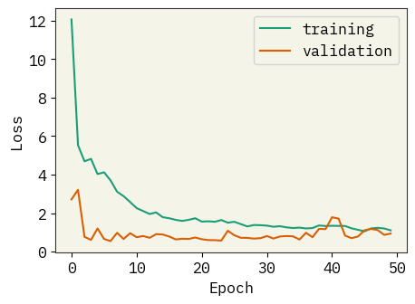
result = model.fit(train_data, validation_data=val_data, epochs=50, verbose=0)

model.save("solubility-rnn-accurate.keras")
# model = tf.keras.models.load_model('solubility-rnn-accurate.keras')

plt.figure(figsize=(5, 3.5))
plt.plot(result.history["loss"], label="training")
plt.plot(result.history["val_loss"], label="validation")
plt.legend()
plt.xlabel("Epoch")
plt.ylabel("Loss")
plt.savefig("rnn-loss.png", bbox_inches="tight", dpi=300)
plt.show()

yhat = []
test_y = []
for x, y in test_data:
    yhat.extend(model(x).numpy().flatten())
    test_y.extend(y.numpy().flatten())
yhat = np.array(yhat)
test_y = np.array(test_y)

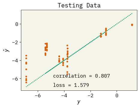
# plot test data
plt.figure(figsize=(5, 3.5))
plt.plot(test_y, test_y, ":")
plt.plot(test_y, yhat, ".")
plt.text(
    max(test_y) - 6,
    min(test_y) + 1,
    f"correlation = {np.corrcoef(test_y, yhat)[0,1]:.3f}",
)
plt.text(
    max(test_y) - 6, min(test_y), f"loss = {np.sqrt(np.mean((test_y - yhat)**2)):.3f}"
)
plt.xlabel(r"$y$")
plt.ylabel(r"$\hat{y}$")
plt.title("Testing Data")
plt.savefig("rnn-fit.png", dpi=300, bbox_inches="tight")
plt.show()

2025-04-06 12:56:06.171318: I tensorflow/core/framework/local_rendezvous.cc:407] Local rendezvous is aborting with status: OUT_OF_RANGE: End of sequence

LIME explanations

In the following example, we find out what descriptors influence solubility of a molecules. For example, let’s say we have a molecule with LogS=1.5. We create a perturbed chemical space around that molecule using stoned method and then use lime to find out which descriptors affect solubility predictions for that molecule.

Wrapper function for RNN, to use in STONED

# Predictor function is used as input to sample_space function
def predictor_function(smile_list, selfies):
    encoded = [selfies2ints(s) for s in selfies]
    # check for nans
    valid = [1.0 if sum(e) > 0 else np.nan for e in encoded]
    encoded = [np.nan_to_num(e, nan=0) for e in encoded]
    padded_seqs = tf.keras.preprocessing.sequence.pad_sequences(encoded, padding="post")
    labels = np.reshape(model.predict(padded_seqs, verbose=0), (-1))
    return labels * valid

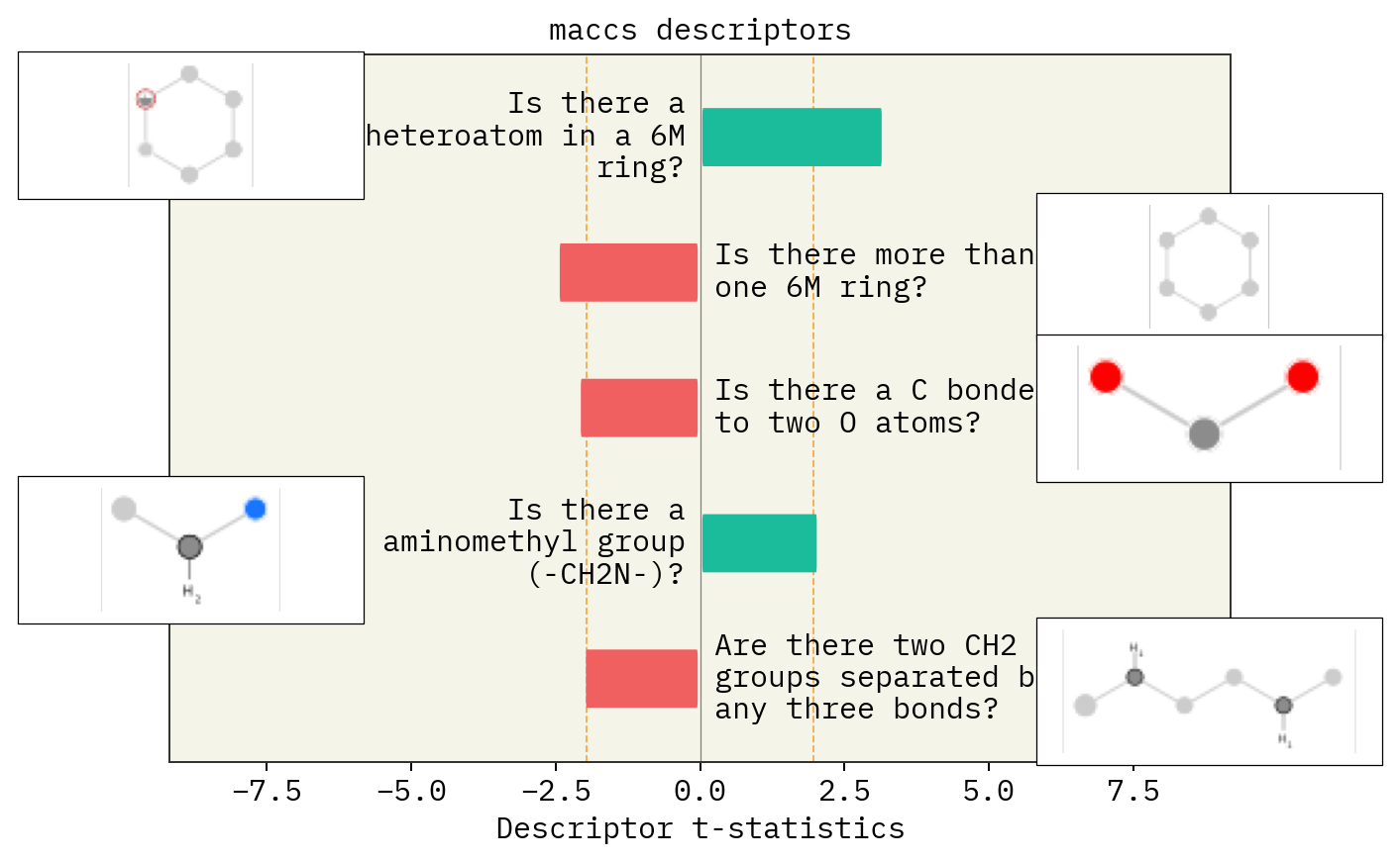
Descriptor explanations

# Make sure SMILES doesn't contain multiple fragments
smi = "CCCCC(=O)N(CC1=CC=C(C=C1)C2=C(C=CC=C2)C3=NN=N[NH]3)C(C(C)C)C(O)=O"  # mol1 - not soluble
# smi = "CC(CC(=O)NC1=CC=CC=C1)C(=O)O" #mol2 - highly soluble
af = exmol.get_basic_alphabet()
stoned_kwargs = {
    "num_samples": 5000,
    "alphabet": af,
    "max_mutations": 2,
}
space = exmol.sample_space(
    smi, predictor_function, stoned_kwargs=stoned_kwargs, quiet=True
)
print(len(space))

4200

from IPython.display import display, SVG

desc_type = ["Classic", "ecfp", "maccs"]

for d in desc_type:
    beta = exmol.lime_explain(space, descriptor_type=d)
    if d == "ecfp":
        display(
            SVG(
                exmol.plot_descriptors(
                    space, output_file=f"{d}_mol2.svg", return_svg=True
                )
            )
        )
        plt.close()
    else:
        exmol.plot_descriptors(space, output_file=f"{d}_mol2.svg")

SMARTS annotations for MACCS descriptors were created using SMARTSviewer (smartsview.zbh.uni-hamburg.de, Copyright: ZBH, Center for Bioinformatics Hamburg) developed by K. Schomburg et. al. (J. Chem. Inf. Model. 2010, 50, 9, 1529–1535)

Text explanations

exmol.lime_explain(space, "ecfp")
s1_ecfp = exmol.text_explain(space, "ecfp")
explanation = exmol.text_explain_generate(s1_ecfp, "aqueous solubility")
print(explanation)

The molecule's aqueous solubility is enhanced by several structural features. The presence of a carbonyl group contributes positively, likely due to its ability to engage in hydrogen bonding with water molecules. Additionally, the inclusion of hetero N basic and nonbasic groups, as well as heteroaromatic groups, further increases solubility by providing sites for hydrogen bonding and dipole-dipole interactions with water. The presence of a primary carbon may enhance solubility by contributing to the overall polarity of the molecule. Furthermore, the n-butyl or amide group also positively influences solubility, possibly through hydrogen bonding or by increasing the molecule's hydrophilic character. If these features were absent, the molecule's aqueous solubility would likely be reduced due to a decrease in potential interactions with water.

Similarity map

beta = exmol.lime_explain(space, "ecfp")
svg = exmol.plot_utils.similarity_map_using_tstats(space[0], return_svg=True)
display(SVG(svg))

# Write figure to file
with open("ecfp_similarity_map_mol2.svg", "w") as f:
    f.write(svg)

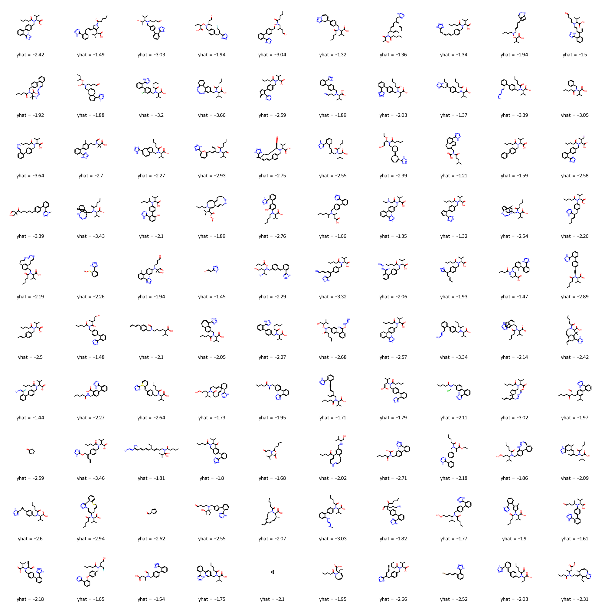
# Inspect space
MolsToGridImage(
    [MolFromSmiles(m.smiles) for m in space],
    legends=[f"yhat = {m.yhat:.3}" for m in space],
    molsPerRow=10,
    maxMols=100,
)

/opt/hostedtoolcache/Python/3.12.9/x64/lib/python3.12/site-packages/rdkit/Chem/Draw/IPythonConsole.py:343: UserWarning: Truncating the list of molecules to be displayed to 100. Change the maxMols value to display more.
  warnings.warn(

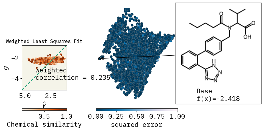
How’s the fit?

fkw = {"figsize": (6, 4)}
font = {"family": "normal", "weight": "normal", "size": 16}

fig = plt.figure(figsize=(10, 5))
mpl.rc("axes", titlesize=12)
mpl.rc("font", size=16)
ax_dict = fig.subplot_mosaic("AABBB")

# Plot space by fit
svg = exmol.plot_utils.plot_space_by_fit(
    space,
    [space[0]],
    figure_kwargs=fkw,
    mol_size=(200, 200),
    offset=1,
    ax=ax_dict["B"],
    beta=beta,
)
# Compute y_wls
w = np.array([1 / (1 + (1 / (e.similarity + 0.000001) - 1) ** 5) for e in space])
non_zero = w > 10 ** (-6)
w = w[non_zero]
N = w.shape[0]

ys = np.array([e.yhat for e in space])[non_zero].reshape(N).astype(float)
x_mat = np.array([list(e.descriptors.descriptors) for e in space])[non_zero].reshape(
    N, -1
)
y_wls = x_mat @ beta
y_wls += np.mean(ys)

lower = np.min(ys)
higher = np.max(ys)

# set transparency using w
norm = plt.Normalize(min(w), max(w))
cmap = plt.cm.Oranges(w)
cmap[:, -1] = w


def weighted_mean(x, w):
    return np.sum(x * w) / np.sum(w)


def weighted_cov(x, y, w):
    return np.sum(w * (x - weighted_mean(x, w)) * (y - weighted_mean(y, w))) / np.sum(w)


def weighted_correlation(x, y, w):
    return weighted_cov(x, y, w) / np.sqrt(
        weighted_cov(x, x, w) * weighted_cov(y, y, w)
    )


corr = weighted_correlation(ys, y_wls, w)

ax_dict["A"].plot(
    np.linspace(lower, higher, 100), np.linspace(lower, higher, 100), "--", linewidth=2
)
sc = ax_dict["A"].scatter(ys, y_wls, s=50, marker=".", c=cmap, cmap=cmap)
ax_dict["A"].text(max(ys) - 3, min(ys) + 1, f"weighted \ncorrelation = {corr:.3f}")
ax_dict["A"].set_xlabel(r"$\hat{y}$")
ax_dict["A"].set_ylabel(r"$g$")
ax_dict["A"].set_title("Weighted Least Squares Fit")
ax_dict["A"].set_xlim(lower, higher)
ax_dict["A"].set_ylim(lower, higher)
ax_dict["A"].set_aspect(1.0 / ax_dict["A"].get_data_ratio(), adjustable="box")
sm = plt.cm.ScalarMappable(cmap=plt.cm.Oranges, norm=norm)
cbar = plt.colorbar(sm, orientation="horizontal", pad=0.15, ax=ax_dict["A"])
cbar.set_label("Chemical similarity")
plt.tight_layout()
plt.savefig("weighted_fit.svg", dpi=300, bbox_inches="tight", transparent=False)

/tmp/ipykernel_41935/2076087530.py:60: UserWarning: No data for colormapping provided via 'c'. Parameters 'cmap' will be ignored
  sc = ax_dict["A"].scatter(ys, y_wls, s=50, marker=".", c=cmap, cmap=cmap)

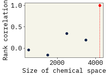
Robustness to incomplete sampling

We first sample a reference chemical space, and then subsample smaller chemical spaces from this reference. Rank correlation is computed between important descriptors for the smaller subspaces and the reference space.

# Sample a big space
stoned_kwargs = {
    "num_samples": 5000,
    "alphabet": exmol.get_basic_alphabet(),
    "max_mutations": 2,
}
space = exmol.sample_space(
    smi, predictor_function, stoned_kwargs=stoned_kwargs, quiet=True
)
len(space)

4201

# get descriptor attributions
exmol.lime_explain(space, "MACCS", return_beta=False)

# Assign feature ids for rank comparison
features = features = {
    a: b
    for a, b in zip(
        space[0].descriptors.descriptor_names,
        np.arange(len(space[0].descriptors.descriptors)),
    )
}

# Get set of ranks for the reference space
baseline_imp = {
    a: b
    for a, b in zip(space[0].descriptors.descriptor_names, space[0].descriptors.tstats)
    if not np.isnan(b)
}
baseline_imp = dict(
    sorted(baseline_imp.items(), key=lambda item: abs(item[1]), reverse=True)
)
baseline_set = [features[x] for x in baseline_imp.keys()]

# Get subsets and calculate lime importances - subsample - get rank correlation
from scipy.stats import spearmanr

plt.figure(figsize=(4, 3))
N = len(space)
size = np.arange(500, N, 1000)
rank_corr = {N: 1}
for i, f in enumerate(size):
    # subsample space
    rank_corr[f] = []
    for _ in range(10):
        # subsample space of size f
        idx = np.random.choice(np.arange(N), size=f, replace=False)
        subspace = [space[i] for i in idx]
        # get desc attributions
        ss_beta = exmol.lime_explain(subspace, descriptor_type="MACCS")
        ss_imp = {
            a: b
            for a, b in zip(
                subspace[0].descriptors.descriptor_names, subspace[0].descriptors.tstats
            )
            if not np.isnan(b)
        }
        ss_imp = dict(
            sorted(ss_imp.items(), key=lambda item: abs(item[1]), reverse=True)
        )
        ss_set = [features[x] for x in ss_imp.keys()]
        # Get ranks for subsampled space and compare with reference
        ranks = {a: [b] for a, b in zip(baseline_set[:5], np.arange(1, 6))}
        for j, s in enumerate(ss_set):
            if s in ranks:
                ranks[s].append(j + 1)
        # compute rank correlation
        r = spearmanr(np.arange(1, 6), [ranks[x][1] for x in ranks])
        rank_corr[f].append(r.correlation)

    plt.scatter(f, np.mean(rank_corr[f]), color="#13254a", marker="o")

plt.scatter(N, 1.0, color="red", marker="o")
plt.axvline(x=N, linestyle=":", color="red")
plt.xlabel("Size of chemical space")
plt.ylabel("Rank correlation")
plt.tight_layout()
plt.savefig("rank correlation.svg", dpi=300, bbox_inches="tight")

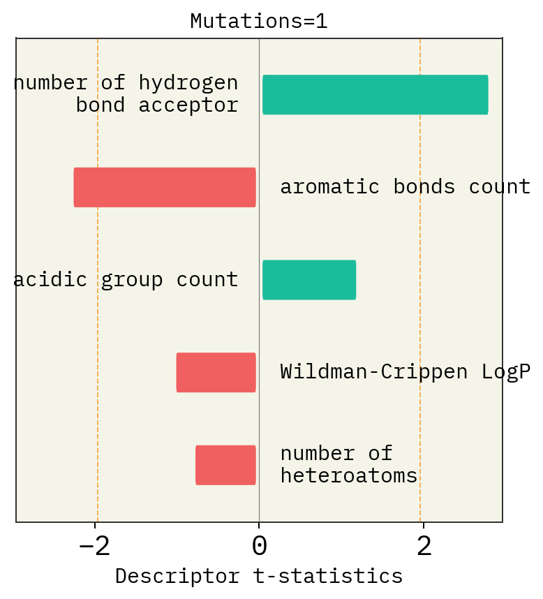
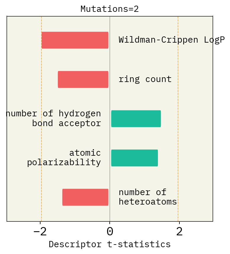
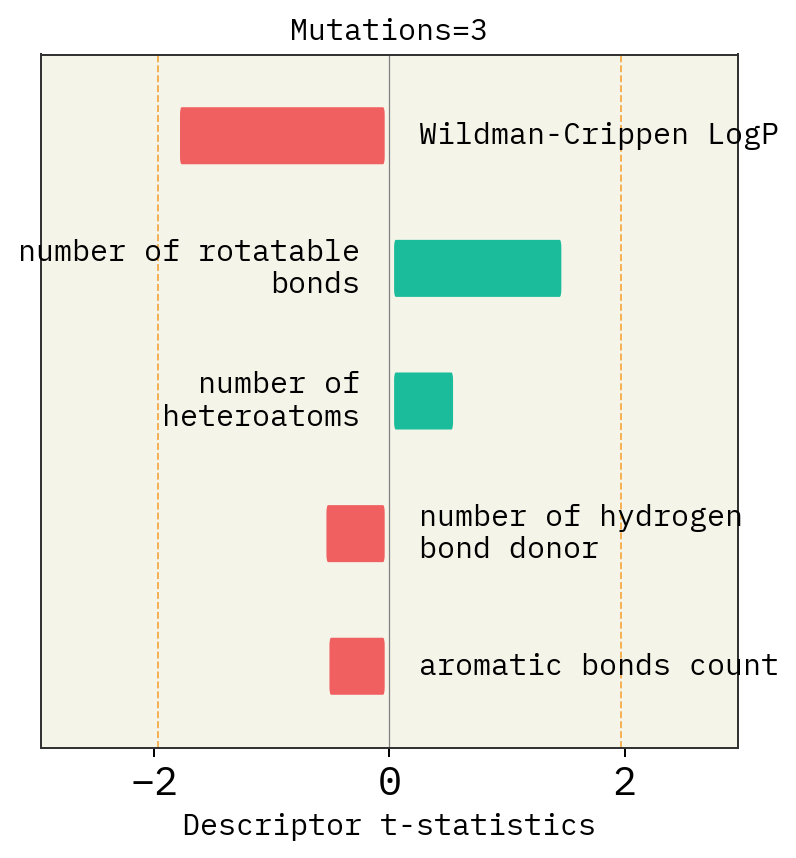
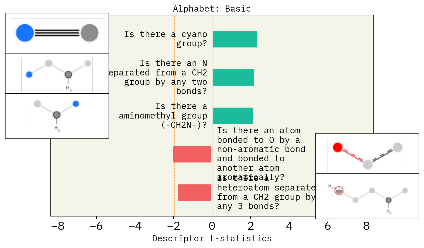
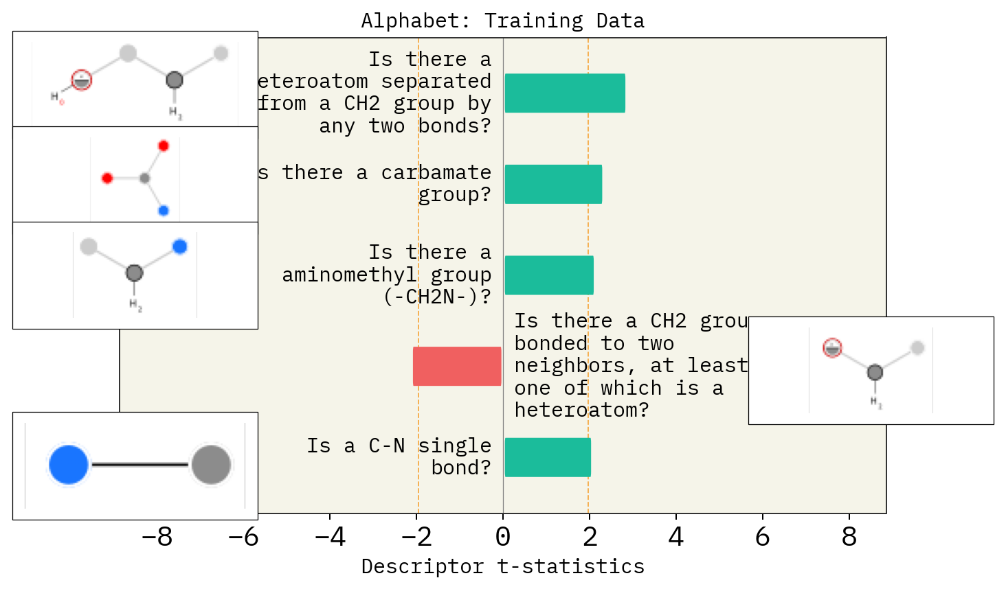
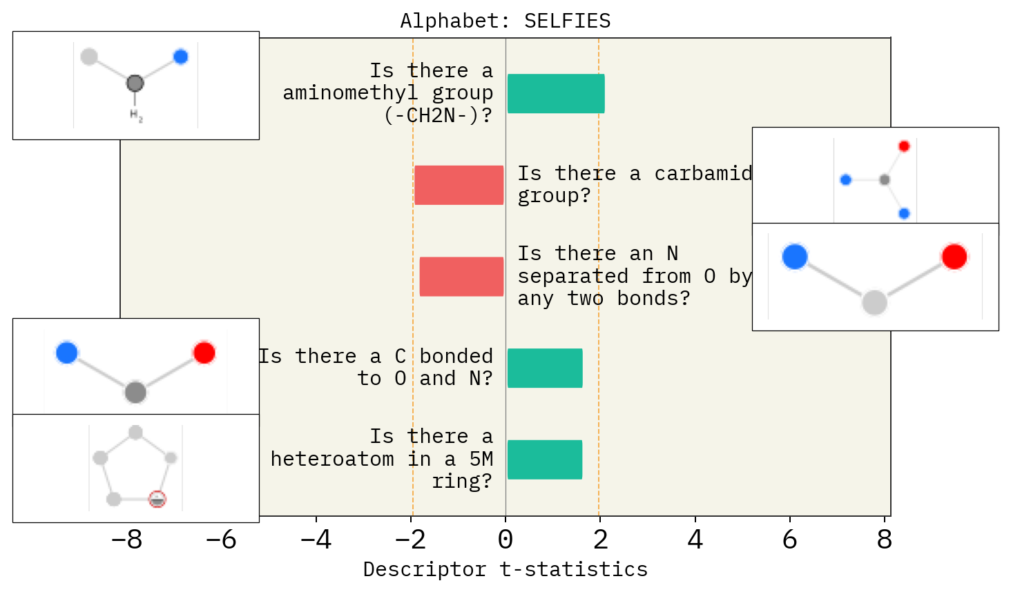
Effect of mutation number, alphabet and size of chemical space

# Mutation
desc_type = ["Classic"]
muts = [1, 2, 3]
for i in muts:
    stoned_kwargs = {
        "num_samples": 2500,
        "alphabet": exmol.get_basic_alphabet(),
        "min_mutations": i,
        "max_mutations": i,
    }
    space = exmol.sample_space(
        smi, predictor_function, stoned_kwargs=stoned_kwargs, quiet=True
    )
    for d in desc_type:
        exmol.lime_explain(space, descriptor_type=d)
        exmol.plot_descriptors(space, title=f"Mutations={i}")

# Alphabet
basic = exmol.get_basic_alphabet()
train = sf.get_alphabet_from_selfies([s for s in selfies_list if s is not None])
wide = sf.get_semantic_robust_alphabet()
desc_type = ["MACCS"]
alphs = {"Basic": basic, "Training Data": train, "SELFIES": wide}
for a in alphs:
    stoned_kwargs = {"num_samples": 2500, "alphabet": alphs[a], "max_mutations": 2}
    space = exmol.sample_space(
        smi, predictor_function, stoned_kwargs=stoned_kwargs, quiet=True
    )
    for d in desc_type:
        exmol.lime_explain(space, descriptor_type=d)
        exmol.plot_descriptors(space, title=f"Alphabet: {a}")

SMARTS annotations for MACCS descriptors were created using SMARTSviewer (smartsview.zbh.uni-hamburg.de, Copyright: ZBH, Center for Bioinformatics Hamburg) developed by K. Schomburg et. al. (J. Chem. Inf. Model. 2010, 50, 9, 1529–1535)

SMARTS annotations for MACCS descriptors were created using SMARTSviewer (smartsview.zbh.uni-hamburg.de, Copyright: ZBH, Center for Bioinformatics Hamburg) developed by K. Schomburg et. al. (J. Chem. Inf. Model. 2010, 50, 9, 1529–1535)

SMARTS annotations for MACCS descriptors were created using SMARTSviewer (smartsview.zbh.uni-hamburg.de, Copyright: ZBH, Center for Bioinformatics Hamburg) developed by K. Schomburg et. al. (J. Chem. Inf. Model. 2010, 50, 9, 1529–1535)

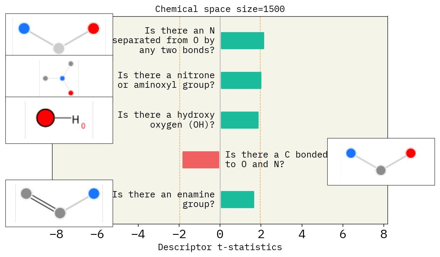
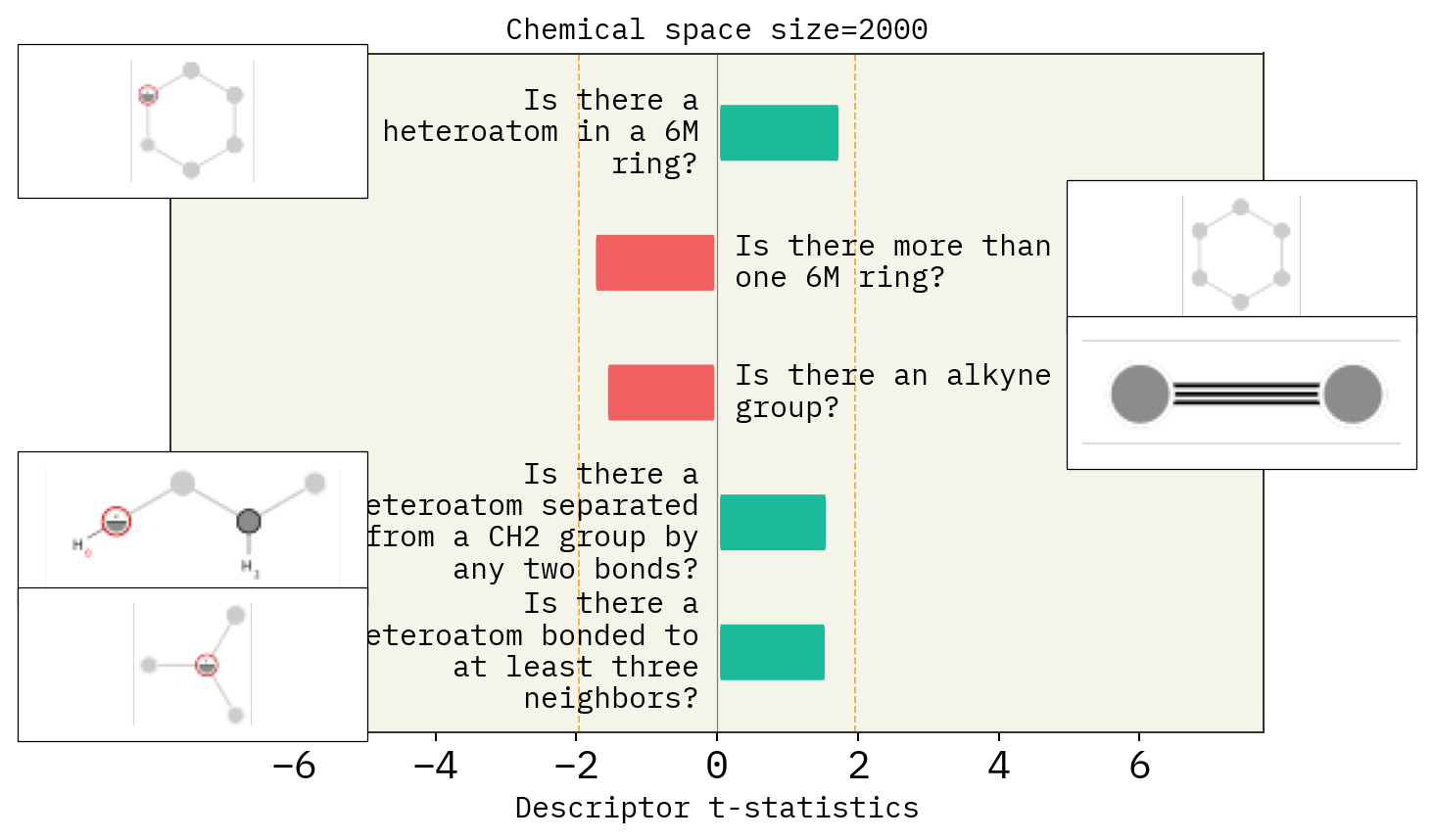
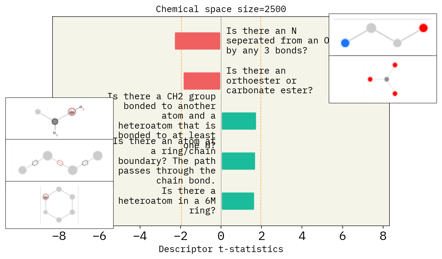
# Size of space
desc_type = ["MACCS"]
space_size = [1500, 2000, 2500]
for s in space_size:
    stoned_kwargs = {
        "num_samples": s,
        "alphabet": exmol.get_basic_alphabet(),
        "max_mutations": 2,
    }
    space = exmol.sample_space(
        smi, predictor_function, stoned_kwargs=stoned_kwargs, quiet=True
    )
    for d in desc_type:
        exmol.lime_explain(space, descriptor_type=d)
        exmol.plot_descriptors(
            space,
            title=f"Chemical space size={s}",
        )

SMARTS annotations for MACCS descriptors were created using SMARTSviewer (smartsview.zbh.uni-hamburg.de, Copyright: ZBH, Center for Bioinformatics Hamburg) developed by K. Schomburg et. al. (J. Chem. Inf. Model. 2010, 50, 9, 1529–1535)

SMARTS annotations for MACCS descriptors were created using SMARTSviewer (smartsview.zbh.uni-hamburg.de, Copyright: ZBH, Center for Bioinformatics Hamburg) developed by K. Schomburg et. al. (J. Chem. Inf. Model. 2010, 50, 9, 1529–1535)

SMARTS annotations for MACCS descriptors were created using SMARTSviewer (smartsview.zbh.uni-hamburg.de, Copyright: ZBH, Center for Bioinformatics Hamburg) developed by K. Schomburg et. al. (J. Chem. Inf. Model. 2010, 50, 9, 1529–1535)